
A real-estate market is more specific than a city on a “best places to invest” list. A growing metropolitan area can contain neighborhoods with very different rents, housing supply and ownership costs. Even on the same street, a renovated house and an older apartment may compete for different occupants.
Useful market research connects three things: the economic activity that supports housing demand, the homes available to meet it, and the choices facing a particular renter or buyer. The aim is to understand where a property fits—and which assumptions about its appeal can be supported.

First, understand what market research can and cannot answer
A real-estate investment depends on both the property and the market around it. The property determines the space, condition and operating plan an investor can offer. The market determines which households or businesses might use it, which alternatives they can choose and the prices and concessions those alternatives require. Research connects those two levels; it does not turn broad population or employment growth into a property-specific forecast.
Four questions organize the work: who creates demand, what competing space exists, what occupants are actually paying and what ownership costs are specific to the location. Public data can describe the first two at a broad level. Listings, completed leases, local records and property-level investigation are needed to test the latter two.
The result should be a bounded assessment with sources, dates and downside cases—not a declaration that a city is simply “good” or “bad.”
Define the market you mean
Begin with the property and its intended use. “A three-bedroom rental house within a practical commute of these employment centers” is a more useful research question than “Is this city a good investment?” It tells you which locations, property types and rental listings belong in the comparison.
Administrative boundaries and housing choices do not always match. County data may describe employment well but combine several distinct rental areas. A ZIP code can include homes with different access, age and condition. Draw an initial search area around the places someone could reasonably consider as alternatives, then adjust it as the evidence becomes clearer.
Keep a short record of the geography, property type, intended use and observation period. This prevents a common analytical mistake: combining a metro-wide growth figure, a county rent estimate and a few premium listings as though they described the same market.
Worked example: We will evaluate a three-bedroom rental house in a fictional county. All example locations, job counts, housing counts and lease offers below are invented for teaching; they are not a market forecast or Faundare loan terms.
Understand the sources of housing demand
Population growth is a starting point. To understand housing demand, also investigate household formation, employment and the types of housing people can obtain. Additional residents do not translate automatically into demand for the particular homes you intend to own.
The Bureau of Labor Statistics’ Quarterly Census of Employment and Wages provides employment and wage information by industry at county and state levels.2 Look at the composition as well as the total: growth spread across several industries tells a different story from expansion concentrated in one employer-dependent sector. The data describe a past period and arrive with a lag; check the reference quarter before calling a trend current.
For households and housing characteristics, the Census Bureau’s American Community Survey can add context. Its estimates have margins of error. The Bureau’s comparison guidance cautions against treating different estimate types and overlapping multiyear periods as interchangeable.3 A small movement in an estimate is not automatically a meaningful change.
Use these sources to form questions for local investigation. If employment has expanded, where are the jobs, when did the expansion occur, and which housing areas offer practical access? If an employer has announced a project, distinguish announced positions from workers already employed. An announcement may justify monitoring an area; it does not establish today's rental demand.
Make the employment comparison reproducible
For a county-level QCEW comparison, select the same county, total industry and ownership coverage for both years. Use annual average employment for a full-year comparison, or the same month in each year to limit seasonal distortion. Save the series selections and release date with the values. Annual and monthly employment are available in QCEW.2
In our fictional county, annual average employment rises from 48,000 to 52,000 over two years: (52,000 ÷ 48,000 − 1) × 100 = 8.3%. That establishes growth in covered jobs in the example. To connect it to this house, investigate commuting patterns, household formation and competing housing. Jobs cannot be converted one-for-one into new renter households.
Look at the homes competing for that demand
Demand becomes more informative when considered alongside supply. A growing area can still offer renters many choices if a large supply pipeline of similar housing becomes available. Conversely, limited new construction does not prove scarcity if existing homes remain vacant or are being converted to rentals.
Separate the development pipeline into projects that are proposed, permitted, under construction and available for occupancy. Those stages represent different levels of commitment and timing. The Census Bureau’s Building Permits Survey measures housing units authorized by permits.4 A permit is not a completed home. Its New Residential Construction releases distinguish authorizations, starts and completions at national and regional levels.5
For a neighborhood, supplement the broader data with planning records, permit information and visible construction. Identify the type of housing being added. A new luxury apartment community and modest detached rental houses are not identical competitors, although price concessions may bring some renters' choices closer together.
Timing matters. A project delivering next month may influence your initial leasing period; a proposed development without a clear schedule belongs in a longer-term watch list. Record its status and source instead of treating every announced unit as imminent competition. Its eventual absorption should be observed rather than assumed.
In the fictional county, housing authorizations rise from 260 to 680 units a year while employment grows. The useful follow-up is to identify which projects compete with the subject home and when they will open. County totals cannot reveal neighborhood vacancy or leasing speed.
Suppose local records and a site visit identify 60 similar rental houses under construction near the subject property, with an expected opening during its first leasing year. Track those homes separately from proposed apartments without a construction date. The 60 homes are part of the broader pipeline, not an extra quantity to add to the county permit total. Their eventual asking rents and concessions could affect this property's initial lease offer.
Read listings as evidence, not just price points
Build a comparable-property set around meaningful similarities: size, layout, condition, parking, amenities and access. Keep genuinely competing properties separate from nearby homes that serve a different need. A large sample of weak comparisons can be less useful than a smaller set whose differences you understand.
For rentals, record the advertised rent, lease term, concessions, required recurring charges and what the rent includes. Date each observation. An asking rent shows what an owner is seeking; it does not prove a tenant agreed to pay it. Where reliable achieved-rent evidence is unavailable, keep that uncertainty visible.
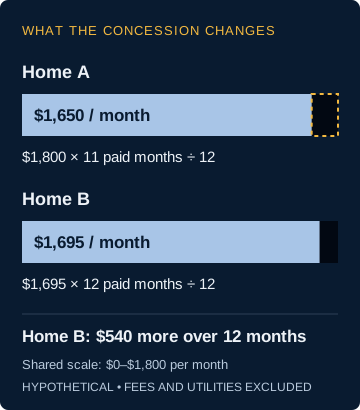
The higher advertised rent can produce less income
Compare two otherwise similar homes over a 12-month lease. Home A offers one month free; Home B offers no concession. Divide total rent due over the lease by 12 to compare the monthly amounts. These fictional offers exclude fees and utilities.
Choose the evidence before choosing the rent
Extend the example to a 1,450-square-foot house with three bedrooms, two bathrooms, a garage and updated interiors. The following fictional evidence log is dated September 15, 2026. Homes A and B above are active offers; the additional entries show how completed leases would change the analysis. All homes use 12-month terms, with the same tenant-paid utilities and no mandatory recurring fees in this example.
| Home / evidence | Comparison with subject | Monthly rent after concessions | Treatment |
|---|---|---|---|
| A / active offer, Sep. 15 | 3 bed, 2 bath; 1,460 sq. ft.; similar updates and garage | $1,650 | Current competition |
| B / active offer, Sep. 15 | 3 bed, 2 bath; 1,420 sq. ft.; similar updates and garage | $1,695 | Current competition |
| C / assumed executed lease, Aug. 20 | 3 bed, 2 bath; 1,430 sq. ft.; similar condition and access | $1,675; no concession | Primary rent evidence |
| D / assumed executed lease, Sep. 1 | 3 bed, 2 bath; 1,480 sq. ft.; similar condition and access | $1,700; no concession | Primary rent evidence |
| E / active offer, Sep. 15 | 4 bed, 3 bath; 2,100 sq. ft.; newly built | $2,200 | Exclude: different product |
Fictional teaching records, not actual leases or property listings. Download the example evidence log (CSV).
C and D bracket a monthly rent of $1,675–$1,700 for similar homes. Their midpoint is $1,687.50, but averaging does not eliminate uncertainty. For this example, use $1,675 per month as the base planning rent, giving more weight to the lower completed lease because the subject will also face A’s concession and the incoming development. Use $1,650 as a separate downside case. These are reasoned scenario choices, not a statistical estimate or appraisal.
Exclude E before calculating an average. Its additional bedroom, larger area and new construction make an unsupported dollar adjustment less defensible than omission. For C and D, the small size differences do not justify inventing a price-per-square-foot adjustment. A real adjustment needs evidence that tenants pay for that difference.
For resale properties, distinguish active listings from closed transactions. Asking prices reveal current competition; documented sales provide evidence of transactions that actually occurred. Examine sale dates, condition and known concessions before using a sale as support for the value of a finished renovation.
Investigate how the neighborhood works
A map can locate a property without explaining the experience of living there. Visit at different times when feasible. Observe access, traffic, noise, property condition and the location of everyday services. Test an expected commute at a relevant time rather than measuring distance alone.
Speak with people who work in the area—property managers, leasing agents, contractors and local planning staff—but ask concrete questions. Which comparable homes have leased recently? What work commonly delays a turnover? Which nearby projects have actually started? Specific observations are easier to verify than claims that a neighborhood is “hot.”
Check what it costs to own this property here
Two locations with similar rents can produce different ownership economics. Obtain property-specific insurance estimates, investigate the local tax assessment process and identify association charges or owner-paid services. A seller's current bill may reflect circumstances that will not apply to a new owner; verify the relevant rules and property record rather than assuming the amount carries forward.
Review physical exposure as well. The FEMA Flood Map Service Center is a source for official flood-hazard mapping.6 Use it alongside property records, inspections and insurance advice; a map lookup is not a complete assessment of a property's condition or insurability.
For the intended rental use, check local requirements with the responsible authority. Registration, inspections, zoning and restrictions on certain rental arrangements depend on jurisdiction and property. This investigation may change the practical use of a home even when the surrounding rental market appears attractive.
Turn the evidence into a market assessment
The market assessment should change an assumption or resolve a choice. Here is the completed conclusion for the fictional rental house.
Completed research memo — fictional example
Revise the rent assumption before proceeding
Market position. Similar completed leases support the base planning rent; active offers and 60 incoming rental homes create pressure on the first leasing period. Employment growth supports the broader demand context but does not justify a premium for this house.
Decision. Replace the original assumption of $1,800 per month with $1,675. That reduces annual scheduled rent by $1,500, from $21,600 to $20,100. At $1,650, scheduled rent would be $19,800. These amounts precede vacancy, expenses and debt service.
How the $20,700 hurdle is calculated
Assume the following annual cash budget at the seller’s price. Each amount is an invented input, not a typical expense estimate.
| Annual cash-budget component | Amount |
|---|---|
| Operating expenses | $7,200 |
| Capital-replacement reserve | $1,800 |
| Debt service | $7,200 |
| Desired cash remaining after those costs | $3,000 |
| Vacancy and collection-loss allowance | $1,500 |
| Required annual scheduled rent | $20,700 |
The $1,500 loss allowance is a fixed-dollar assumption for this comparison, not a vacancy-rate estimate. Holding these inputs constant, the $20,100 base rent leaves $2,400 after allowances and costs—$600 short of the target. The downside case leaves $2,100, a $900 shortfall. This is a cash-budget test before income tax; reserve funding is included as a cash allocation.
Consequence for this candidate. Neither scenario meets the investor’s $3,000 cash target at the seller’s price. Revise the acquisition price and financing model or reject the candidate; raising the rent assumption would contradict the selected comparables. The target is an illustrative investor preference, not a lending requirement.
Reassessment trigger. Reopen the rent conclusion if comparable executed leases change, the subject’s condition changes, or the competing development begins leasing on materially different terms. A price reduction alone changes acquisition economics, not the evidence for rent.
References
1. Breno Assis. Aerial view of suburban neighborhood houses. https://unsplash.com/photos/aerial-view-of-suburban-neighborhood-houses-r3WAWU5Fi5Q. Unsplash. Used under the Unsplash License. Accessed October 3, 2026.
References are numbered in order of first citation. Access dates identify the versions consulted; these maintained web resources are cited without an inferred publication year.
2. U.S. Bureau of Labor Statistics. QCEW Overview. https://www.bls.gov/cew/overview.htm. Accessed September 24, 2026.
3. U.S. Census Bureau. Comparing ACS Data. https://www.census.gov/programs-surveys/acs/guidance/comparing-acs-data.html. Accessed September 24, 2026.
4. U.S. Census Bureau. Building Permits Survey. https://www.census.gov/construction/bps/index.html. Accessed September 24, 2026.
5. U.S. Census Bureau. New Residential Construction. https://www.census.gov/construction/nrc/index.html. Accessed September 24, 2026.
6. Federal Emergency Management Agency. Flood Map Service Center. https://msc.fema.gov/portal/home. Accessed September 24, 2026.
Figure and table provenance. The analytical figure, calculations and example data were created by Faundare Capital for this guide. The opening photograph is cited in the references. Government references support the research methods and data definitions; they do not supply the fictional observations.